Digitalna transformacija šumarstva kroz praktične GIS tutorijale
U vremenu kada se šumarstvo sve više oslanja na podatke iz dronova, LiDAR skenere i satelitske slike, sve veća je potreba za pristupačnim izvorima znanja koji spajaju tehnologiju i prirodu. Jedan od takvih izvora, koji zaslužuje posebno mjesto na blogu ForestryTech, jeste YouTube kanal Maps by RGD.
Autor kanala, Rúben Duarte, donosi praktične video tutorijale iz oblasti GIS-a, daljinske detekcije (Remote Sensing) i prostorne analize, s naglaskom na stvarne, terenske primjene — od mapiranja šuma do procjene biomase i ugljika. Kanal broji više od 300 videa i privlači sve veći broj profesionalaca i studenata koji žele savladati geoinformacione tehnologije kroz realne projekte.
U nastavku izdvajamo dva izuzetno korisna videa koji su posebno relevantni za profesionalce u šumarstvu i srodnim ekološkim oblastima.
LiDAR u službi prepoznavanja strukture šume
LiDAR u službi prepoznavanja strukture šume
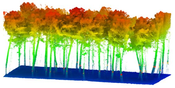
U ovom videu, Rúben Duarte detaljno objašnjava postupak izdvajanja stabala iz LiDAR podataka pomoću ArcGIS Pro.
Cilj je jednostavan, ali tehnološki zahtjevan — identifikovati pojedinačna stabla iz oblaka tačaka (point cloud) kako bi se mogao analizirati šumski sklop i struktura krošnji.
Tehnički pristup:
- Korištenje LAS dataset-a (LiDAR datoteka) u ArcGIS Pro.
- Generisanje Digital Surface Model (DSM) i Canopy Height Model (CHM).
- Primjena alata za Tree Extraction koji prepoznaje visinske vrhove (local maxima) kao indikatore stabala.
- Vizuelizacija rezultata i provjera tačnosti ekstrakcije.
Zašto je ovo važno za šumarstvo:
Izdvajanje stabala iz LiDAR podataka postalo je temelj savremene inventarizacije šuma. Umjesto tradicionalnih terenskih metoda koje zahtijevaju mnogo vremena i resursa, LiDAR omogućava dobijanje detaljnih strukturalnih informacija o visini, gustoći i rasporedu stabala — i to s visokom preciznošću.
Ovaj tutorijal je izuzetno koristan za:
- dron-operatere i GIS analitičare koji rade s LiDAR podacima iz zraka,
- istraživače biomase koji žele izdvojiti pojedinačne krošnje kao bazu za dalju analizu,
- projektne timove koji se bave restauracijom šuma ili mapiranjem degradiranih područja.
Posebno je zanimljivo što autor koristi standardne ArcGIS Pro alate, bez potrebe za dodatnim skriptama — čineći proces transparentnim i ponovljivim.
Takav pristup omogućava jednostavnu primjenu i u BiH, gdje LiDAR i drone podaci sve češće postaju dostupni u projektima pošumljavanja i inventarizacije.
Od visine stabla do ugljika: kako QGIS postaje alat za klimatske analize
U drugom videu, Duarte prelazi korak dalje – pokazuje kako iz istih LiDAR podataka možemo izračunati biomasu (AGB) i ugljik (C), koristeći otvoreni alat QGIS.
Ovaj proces omogućava šumarskim stručnjacima da kvantifikuju ekološku vrijednost svojih šuma – koliko ugljika je pohranjeno u vegetaciji, koliki je prirast i kako se taj kapacitet mijenja kroz vrijeme.
Koraci iz videa:
- Učitavanje i obrada LiDAR podataka (LAS/LAZ format).
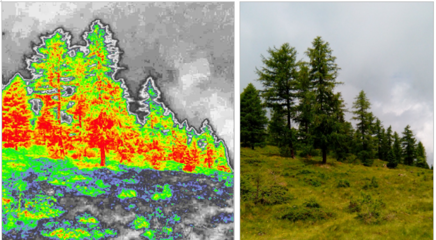
- Izrada CHM (Canopy Height Model) – model visine krošnje koji služi kao osnova za izračune.
- Identifikacija pojedinačnih stabala i procjena visine.
- Primjena empirijskih formula za proračun biomase i ugljika.
Formula koju autor koristi povezuje visinu i volumen stabla s poznatim faktorima gustoće drveta, dajući procjenu količine suhe biomase, a zatim i ugljika (obično oko 0.47 × AGB).
Pristup koji Rúben Duarte koristi je izuzetno vrijedan jer:
- demonstrira otvoreni softver (QGIS) – pristupačan svima, bez troškova licenci,
- povezuje LiDAR podatke s ekološkim pokazateljima,
- omogućava kvantifikaciju učinka pošumljavanja u realnim brojkama (tone biomase i ugljika po hektaru).
Ovaj autor uz svoje tutorijale dijeli i kompletan materijal na svom G-Disku, čime vam omogućava da dodatno dorađujete predstavljene modele i da ih koriste u vlastitim projektima.
Za šumarske inženjere i GIS stručnjake u Bosni i Hercegovini i regionu, ovaj metod može poslužiti kao baza za razvoj lokalnih modela biomase.
Posebno kada se kombinuje s dron-snimcima, moguće je razviti kompletan digitalni sistem nadzora šumskog rasta i koncentracije uskladištenog ugljika – što je upravo smjer ka kojem ide moderna šumarska tehnologija i projekti koji su široko podržani od strane različitih EU i Globalnih Fondova.